Vectors ☰

Vectors are mathematical objects that are commonly used in various fields of science, engineering, and mathematics. They are used to represent physical quantities such as force, velocity, acceleration, and displacement that have both magnitude and direction.
A vector is usually represented by an arrow with a length and a direction. The length of the arrow represents the magnitude of the vector, while the direction of the arrow represents the direction of the vector. The magnitude of a vector is a scalar value and is denoted by \( \vec{|v|} \).
Vectors can be denoted by naming their start and end points, where the start point is the tail of the vector and the end point is the head of the vector. For example, the vector from point \(A\) to point \(B\) can be denoted as \( \overrightarrow{AB} \) .

Vectors have a number of properties that are important in mathematics and physics. Some of the key properties of vectors include:

Magnitude: Vectors have a magnitude or length, which is a non-negative scalar that represents the size of the vector.

Direction: Vectors have a direction, which can be specified using angles or other directional notations. The direction of a vector is defined by the angle between the vector and a fixed reference direction.

Addition: Vectors can be added together using the parallelogram law or the triangle law of vector addition. This involves adding the corresponding components of each vector to obtain the resulting vector.

Scalar multiplication: Vectors can be multiplied by scalars, which changes the magnitude and/or direction of the vector. Scalar multiplication involves multiplying each component of the vector by a scalar.

Dot product: Vectors can be multiplied together using the dot product or scalar product. The dot product of two vectors is a scalar that represents the product of their magnitudes and the cosine of the angle between them.

Cross product: Vectors can also be multiplied using the cross product or vector product. The cross product of two vectors is a vector that is perpendicular to both input vectors and has a magnitude equal to the product of their magnitudes times the sine of the angle between them.

Zero vector: There is a unique vector called the zero vector, denoted by \( \vec{0} \), which has a magnitude of \(0\) and no direction. It can be thought of as the vector that goes from a point to itself, or equivalently, as the difference between any two equal vectors.
For example, \( \overrightarrow{OA} - \overrightarrow{OA} = 0 \).

Unit vector: A unit vector is a vector with a magnitude of 1. Any non-zero vector can be divided by its magnitude to obtain a unit vector in the same direction.

Collinear vectors: Vectors are collinear if they lie on the same line or are parallel. In other words, they have the same or opposite direction. Collinear vectors can be written as scalar multiples of each other. If two vectors \( \vec{v} \) and \( \vec{w} \) are collinear, then there exists a scalar \(k\) such that \( \vec{v} = k \vec{w} \) or \( \vec{w} = k \vec{v} \). This means that one vector is a scalar multiple of the other, and they point in the same or opposite directions.

Orthogonal vectors: Two vectors are orthogonal if their dot product is zero. Orthogonal vectors are also called perpendicular vectors, and they form a 90-degree angle between them.

Basis vectors: A set of basis vectors is a set of linearly independent vectors that can be used to represent any other vector in a space. The most common basis vectors are the standard unit vectors in three-dimensional space, which are denoted by \(\hat{i}\) , \( \hat{j} \) and \( \hat{k} \).

Linear independence: A set of vectors is linearly independent if none of the vectors in the set can be expressed as a linear combination of the others. If a set of vectors is linearly independent, then it can be used as a basis for a vector space.

Span: The span of a set of vectors is the set of all linear combinations of those vectors. The span of a set of vectors is a subspace of the vector space containing those vectors.

Projection: The projection of one vector onto another is the component of the first vector that lies in the direction of the second vector. The projection of vector \( \vec{u} \) onto vector \(\vec{v}\) is given by $$ \text{proj}_{\vec{v}} ( \vec{u} ) = \frac{\vec{u} \cdot v}{||\vec{v}||^2} \vec{v} $$

Component: The component of one vector along another is the part of the first vector that lies in the direction of the second vector. The component of vector \( \vec{u} \) along vector \( \vec{v} \) is given by $$ \text{comp}_{\vec{v}} (\vec{u}) = \frac{\vec{u} \cdot v}{||\vec{v}||^2} cos \theta $$ where \(\theta \) is the angle between \(\vec{u} \) and \(\vec{v} \).

Parallel transport: Parallel transport is a way of moving vectors along a curve in a way that preserves their direction. Parallel transport is used in differential geometry and other fields to study the curvature of curves and surfaces.

Covariance and contravariance: In mathematics and physics, vectors are often classified as covariant or contravariant based on how their components transform under coordinate transformations. Covariant vectors have components that transform in the same way as the coordinates, while contravariant vectors have components that transform in the opposite way. The concept of covariance and contravariance is used extensively in tensor calculus and other areas of mathematics and physics.

These are just a few of the many properties of vectors.

The length of a vector (Magnitude) ☰

In mathematics, the length of a vector is also known as its magnitude or norm. It represents the distance between the origin and the endpoint of the vector in a geometric space.
For a vector with components \( (x, y, z) \) in a three-dimensional space, its length can be calculated using the following formula: $$ |\vec{v}| = \sqrt{(x^2+ y^2+ z^2 )} $$ In two-dimensional space, the formula for the length of a vector with components \((x, y)\) is: $$ |\vec{v}| = \sqrt{(x^2+ y^2 )} $$ In general, the length of a vector can be calculated using the Pythagorean theorem, which states that the square of the length of the vector is equal to the sum of the squares of its components.

The direction of a vector ☰

The direction of a vector can be determined by calculating its angle with respect to a reference axis. This angle is often measured counterclockwise from the positive direction of the reference axis.
If \( \vec{v} \) is a vector in two-dimensional space with components \( (v_x,v_y ) \), then its direction \( \theta \) is given by: $$ \theta = arctan (\frac{v_y}{v_x} ) $$ where arctan is the inverse tangent function.

In three-dimensional space, a vector \( \vec{v} \) with components \( (v_x,v_y,v_z ) \) can be represented as a directed line segment from the origin \( (0,0,0) \) to the point \( (v_x,v_y,v_z ) \). Its direction can be described by two angles: the azimuthal angle \(\varphi \), which is the angle measured counterclockwise from the positive \(x\)-axis in the \(xy\)-plane and the polar angle \( \theta \), which is the angle measured from the positive \(z\)-axis to the line segment.

The azimuthal angle \( \varphi \) is given by: $$ \varphi = arctan (\frac{v_y}{v_x} ) $$ if \( v_x > 0 \), and $$ \varphi = arctan (\frac{v_y}{v_x} ) + \pi $$ if \( v_x < 0 \), the polar angle \( \theta \) is given by: $$ \theta=arccos ( \frac{v_z}{|\vec{v} |} ) $$ where \( |\vec{v} | \) is the magnitude of the vector \( \vec{v} \).

Another way to describe the direction of a vector in three-dimensional space is to use its direction cosines. The direction cosines of a vector \(\vec{v} \) with components \( (v_x,v_y,v_z ) \) are defined as: $$ \cos\alpha = \frac{v_x}{|\vec{v}|} $$ $$ \cos\beta = \frac{v_y}{|\vec{v}|} $$ $$ \cos\gamma = \frac{v_z}{|\vec{v}|} $$ where \(\alpha \), \( \beta \) and \( \gamma \) are the angles between the vector \( \vec{v} \) and the positive \(x\), \(y\) and \(z\)-axes, respectively.

If the direction cosines of a vector are known, its direction can be determined using the following equations: $$ \small \varphi = \begin{cases} \arccos\left(\frac{\cos\beta}{\sqrt{\cos^2\alpha + \cos^2\beta}}\right) & \text{if } \cos\alpha > 0 \\ 2\pi - \arccos\left(\frac{\cos\beta}{\sqrt{\cos^2\alpha + \cos^2\beta}}\right) & \text{if } \cos\alpha < 0 \end{cases} $$ $$ \theta=arccos(\cos\gamma ) $$ where \( \varphi \) is the azimuthal angle and \( \theta \) is the polar angle.

In addition to these methods, the direction of a vector can also be described using unit vectors. A unit vector is a vector with magnitude 1 that points in the same direction as the original vector. Given a vector \( \vec{v} \), its unit vector \( \hat{v} \) can be calculated as: $$ \hat{v} = \frac{\vec{v} }{\vec{|v|}} $$ Once the unit vector is known, its direction can be described by the angles \( \theta \) and \( \varphi \) as described above.
It's worth noting that the direction of a vector is independent of its magnitude. Therefore, a vector and a scalar multiple of that vector have the same direction.

Addition and Subtraction of Collinear Vectors ☰

Collinear vectors are vectors that lie on the same line. When two collinear vectors are added or subtracted, the result is another collinear vector. The magnitude of the result is the sum or difference of the magnitudes of the two vectors, depending on whether we are adding or subtracting them. The direction of the result is the same as the direction of the two vectors since they are collinear.

Let's say we have two collinear vectors \( \vec{a} \) and \( \vec{b} \), with magnitudes \( \vec{|a|} \) and \( \vec{|b|} \) respectively. If they point in the same direction, their sum is given by: \( \vec{a} + b = ( \vec{|a|} + \vec{|b|} ) \hat{a} \). Where \( \hat{a} \) is the unit vector in the direction of \( \vec{a} \) If they point in opposite directions, their difference is given by: $$ \vec{a} - b = ( \vec{|a|} - \vec{|b|} ) \hat{a} $$

Methods of Addition and Subtraction of Non-Collinear Vectors ☰

Non-collinear vectors are vectors that do not lie on the same line. When adding or subtracting non-collinear vectors, we use the parallelogram law or the triangle law, depending on the situation.

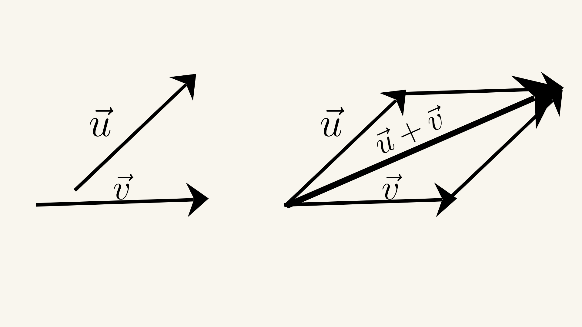
Parallelogram Law
The parallelogram law states that the sum of two vectors can be found by placing the vectors head to tail and drawing the parallelogram formed by the two vectors. The vector sum is the diagonal of the parallelogram that starts from the common point of the two vectors. The parallelogram law can be used to add any number of vectors, not just two. Let's say we have two non-collinear vectors \( \vec{a} \) and \( \vec{b} \). We can find their sum \( \vec{c} \) using the parallelogram law: \( \vec{c} = a+b \).
We first place the tail of vector \( \vec{b} \) at the head of vector \( \vec{a} \) to form a parallelogram. The diagonal of the parallelogram starting from the common point of the two vectors represents the sum vector \( \vec{c} \). The magnitude of the sum vector \( \vec{c} \) can be found using the law of cosines: $$\vec{|c|}^2 = \vec{|a|}^2 + \vec{|b|}^2 + 2 \vec{|a|} \vec{|b|} cos \theta $$ where \( \theta \) is the angle between the vectors \( \vec{a} \) and \( \vec{b} \).


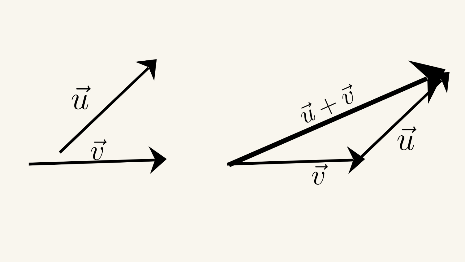
Triangle Law
The triangle law states that the sum of two vectors can be found by placing the vectors head to tail and drawing the third side of the triangle that connects the tail of the first vector to the head of the second vector. The sum vector is the diagonal of the triangle that starts from the common point of the two vectors.
Let's say we have two non-collinear vectors \( \vec{a} \) and \(\vec{b} \). We can find their sum \( \vec{c} \) using the triangle law: \( \vec{c}= a+ b \).
We first place the tail of vector \(\vec{a} \) at the origin and then place the tail of vector \( \vec{b} \) at the head of vector \( \vec{a} \). The sum vector \( \vec{c} \) is the diagonal of the triangle that starts from the origin and connects the head of vector \( \vec{b} \). The magnitude of the sum vector \(\vec{c} \) can be found using the law of cosines: \( |\vec{c} |^2 = |\vec{a} |^2 + |\vec{b}|^2 -2 |\vec{a}| |\vec{b}| cos \theta \), where \( \theta \) is the angle between the vectors \(\vec{a} \) and \(\vec{b}\).
Subtraction of vectors can also be done using either the parallelogram law or the triangle law. To subtract vector \( \vec{b} \) from vector \(\vec{a}\), we simply reverse the direction of vector \( \vec{b} \) and add it to vector \(\vec{a}\) using either the parallelogram law or the triangle law. \( \vec{a} - \vec{b} = \vec{a} + (-\vec{b} ) \)


Properties of Vector Addition
Vector addition has several important properties that make it useful in physics and other fields:

• Commutative Property: The order in which vectors are added does not affect the result. $$ \vec{a} + \vec{b} = \vec{b} + \vec{a} $$
• Associative Property: When adding more than two vectors, the order in which we group the vectors does not affect the result. $$ (\vec{a} + \vec{b}) + \vec{c} = \vec{a} + (\vec{b} + \vec{c}) $$
• Zero Vector: The zero vector \( \vec{0} \), with magnitude zero and any direction, is the additive identity for vectors. Adding the zero vector to any vector does not change the vector. $$ \vec{a} + \vec{0} = \vec{a} $$
• Additive Inverse: For every vector \( \vec{a} \), there exists an additive inverse vector \( -\vec{a} \) such that their sum is the zero vector. $$ \vec{a} + (-\vec{a}) = \vec{0} $$
• Distributive Property: Scalar multiplication distributes over vector addition. $$ (\vec{a} + \vec{b}) = k \vec{a} + k \vec{b} $$ where \(k\) is any scalar.

Adding Vectors Using Components ☰

When adding vectors using components, the first step is to break each vector into its \(x\) and \(y\) components. This can be done using trigonometric functions such as sine and cosine. For example, given a vector with magnitude "\(r\)" and angle "\(\theta \)" with respect to the \(x\)-axis, its \(x\) and \(y\) components can be found as follows:
\(x\)-component: \(r\cdot cos(\theta) \).
\(y\)-component: \(r\cdot sin(\theta) \).

Once both vectors have been broken down into their \(x\) and \(y\) components, the components can be added together separately. For example, if we have two vectors \(A\) and \(B\), their \(x\)-components can be added together to get the \(x\)-component of the resulting vector \(C\), and their \(y\)-components can be added together to get the \(y\)-component of \(C\):
\(C_x = A_x+ B_x \)
\(C_y= A_y+ B_y \)

Finally, the magnitude and angle of vector \(C\) can be found using the Pythagorean theorem and inverse trigonometric functions, respectively:
magnitude of \(C\): \( \sqrt{C_x^2 + C_y^2} \) .
angle of \(C\): \( tg^{-1} \left(\frac{C_y}{C_x} \right) \) .
Note that the angle of C may need to be adjusted based on which quadrant it is in, as inverse trigonometric functions only give angles in the range of \( -\frac{\pi}{2} \) to \( \frac{\pi}{2} \).

To adjust the angle of vector \(\vec{C} \), we need to consider the signs of its \(x\) and \(y\) components. If \(C_x\) and \(C_y\) are both positive, then the angle of C is simply the inverse tangent of \( \frac{C_y}{C_x} \). If \(C_x\) is negative and \(C_y\) is positive, then the angle of \(C\) is 180 degrees minus the inverse tangent of \( \frac{C_y}{|C_x|} \). If \(C_x\) is negative and \(C_y\) is negative, then the angle of \(C\) is 180 degrees plus the inverse tangent of \( \frac{|C_y |}{|C_x |} \). Finally, if \(C_x\) is positive and \(C_y\) is negative, then the angle of \(C\) is 360 degrees minus the inverse tangent of \( \frac{|C_y|}{C_x} \).

For example, suppose we have two vectors \(A\) and \(B\) with magnitudes of 3 and 4, respectively, and angles of 30 degrees and 60 degrees with respect to the \(x\)-axis. We can find the \(x\) and \(y\) components of each vector as follows:
\( A_x = 3 \cdot cos(30) = 2.598 \)
\( A_y = 3 \cdot sin(30)= 1.5 \)
\( B_x = 4 \cdot cos(60)= 2 \)
\( B_y = 4 \cdot sin(60)= 3.464 \)

We can then add the \(x\) and \(y\) components of \(A\) and \(B\) to get the \(x\) and \(y\) components of \(C\):
\( C_x = A_x + B_x= 4.598 \)
\( C_y = A_y + B_y= 4.964 \)

The magnitude of \( \vec{C} \) is:
\( \small \vec{|C|} = \sqrt{C_x^2+ C_y^2} = \sqrt{4.598^2 + 4.964^2} = 6.425 \)

The angle of \(C\) is:
\( \small \theta = tan^{-1} \left(\frac{C_y}{C_x} \right) = tan^{-1} \left(\frac{4.964}{4.598} \right) = 49.1^\circ \)

Since both \(C_x\) and \(C_y\) are positive, this is the final answer. Therefore, the resulting vector \(C\) has a magnitude of 6.425 and an angle of 49.1 degrees with respect to the \(x\)-axis.

Scalar multiplication ☰

Scalar multiplication is the operation of multiplying a vector by a scalar, which is a real number. When a vector is multiplied by a scalar, the magnitude of the vector is scaled by the absolute value of the scalar, and the direction of the vector is unchanged if the scalar is positive, or reversed if the scalar is negative.
Mathematically, scalar multiplication can be expressed as follows: given a vector \(v\) and a scalar \(k\), the scalar multiple of \( \vec{v} \) by \(k\), denoted \( k \cdot \vec{v} \), is a vector with the same direction as \( \vec{v} \) but with magnitude scaled by the absolute value of \(k\):
\( k \cdot \vec{v} = (|k|) \cdot \vec{v} \)

If \(k\) is positive, then the direction of \( k \cdot \vec{v} \) is the same as the direction of \(\vec{v} \). If \(k\) is negative, then the direction of \( k \cdot \vec{v} \) is opposite to the direction of \( \vec{v} \).

Scalar multiplication can be used to stretch or shrink vectors. For example, if we have a vector \( \vec{v} \) that represents a displacement in meters, we can multiply it by a scalar to represent a displacement that is larger or smaller than \( \vec{v} \). Additionally, scalar multiplication can be used to reverse the direction of a vector by multiplying it by \(-1\).

Scalar multiplication can also be used to find linear combinations of vectors. A linear combination of two vectors is simply the sum of the vectors multiplied by scalar coefficients.
For example, given two vectors \( \vec{v} = (2,3) \) and \( \vec{w} = (1,-1) \), the linear combination \( 3 \vec{v} – 2 \vec{w} \) can be computed as follows: $$ \begin{align*} &3\vec{v} = 3(2,3) = (6,9)& \\ &2\vec{w} = 2(1,-1) = (2,-2)& \\ &3\vec{v} - 2\vec{w} = (6,9) - (2,-2) = (4,11)& \end{align*} $$ The resulting vector \((4,11)\) is a linear combination of \( \vec{v} \) and \( \vec{w} \) with coefficients \(3\) and \(-2\), respectively.

Scalar multiplication also satisfies several important properties:

• Distributivity: For any scalars \(k\) and \(l\) and any vector \( \vec{v} \), we have \( (k+l) \vec{v} = k \vec{v} + l \vec{v} \).
• Associativity: For any scalar \(k\) and any vectors \( \vec{u} \) and \( \vec{v} \), we have \( k( \vec{u} + \vec{v} ) = k \vec{u} + k \vec{v} \).
• Compatibility with multiplication: For any scalars \(k\) and \(l\) and any vector \( \vec{v} \), we have \( (kl) \vec{v} = k(l \vec{v}) \).

These properties make scalar multiplication a useful tool for manipulating and solving systems of linear equations.

Parallel transport ☰

Parallel transport is a concept in differential geometry that describes how a vector or a tangent space along a curve can be transported along the curve without changing its direction. It is an important concept in understanding the geometry of curved spaces.

In general, a curve on a manifold is a path that connects two points on the manifold. A tangent vector is a vector that is tangent to the curve at a particular point. Parallel transport along a curve is the process of moving a tangent vector along the curve while keeping it tangent to the curve at each point.

The idea of parallel transport is closely related to the concept of a connection on a manifold. A connection is a way of connecting tangent spaces at different points on a manifold. It allows for the comparison of tangent vectors at different points on a curve.

In order to define parallel transport, one needs to specify a connection on the manifold. Given a connection, the parallel transport of a vector along a curve is defined as the unique vector that is tangent to the curve at each point and whose components in a particular basis remain constant along the curve.

The concept of parallel transport is important in many areas of physics, including general relativity, where it is used to describe the transport of tensors along curved spacetime trajectories.

Transformation and congruent figures ☰

Transformation refers to the process of changing the position, size, or shape of a geometric figure. There are several types of transformations, including translations, reflections, rotations, and dilations. Congruent figures are geometric figures that have the same size and shape, and their corresponding sides and angles are congruent.

Here are some important theorems related to transformations and congruent figures:

• Corresponding parts of congruent figures are congruent (CPCTC): This theorem states that if two figures are congruent, then their corresponding sides, angles, and vertices are congruent.
• The composition of translations is a translation: If two translations are performed one after the other, then the resulting transformation is also a translation.
• The composition of reflections is a rotation or a translation: If two reflections are performed one after the other, then the resulting transformation is either a rotation or a translation.
• The composition of rotations is a rotation: If two rotations are performed one after the other, then the resulting transformation is also a rotation.
• The composition of a dilation and a translation is a dilation: If a dilation and a translation are performed one after the other, then the resulting transformation is also a dilation.
• The composition of a dilation and a rotation is a dilation or a rotation: If a dilation and a rotation are performed one after the other, then the resulting transformation is either a dilation or a rotation.
• The composition of two congruent transformations is a congruent transformation: If two transformations are congruent, then their composition is also congruent.

These theorems are important in understanding the properties of transformations and congruent figures, and they can be used to prove various geometric theorems and solve problems in geometry.